Retrospective Formatting

Changing Plot Axes

Limits

The axes limits in x, y, z or colour can be changed by the commands lx, ly, lz and lc respectively. Colour limits define the lowest and highest values to which colours are allocated. Anything below the lower limit will be the lowest colour and any points above the upper limit will be the highest colour.

>> lx(xlo, xhi)
>> ly(ylo, yhi)
>> lz(zlo, zhi)
>> lc(clo, chi)

• If the selected plot is an area plot then lz and lc both change the colour scale
• lz and lc are not applicable for one dimensional plots
• If no limits are given to a command the following happens:
  • lx - x limits are between the lowest and highest value of x in the data
  • ly - y limits are between the lowest and highest value of y in the data contained within the current x limits
  • lz/lc - z/c limits are between the lowest and highest value of z in the data contained within the current x and y limits

Changing the Scale to Log

The axes scale for x, y, z and colour can be changed to a logarithmic scale using the commands logx, logy, logz and logc respectively.

>> logx
>> logy
>> logz
>> logc

• If the selected plto is an area plot then logz and logc both change the colour scale
• logz and logc are not applicable for one dimensional plots
• If the scale is already logarithmic then nothing happens (i.e. no warning or error is given)

Similarly, the axes scale for x, y, z and colour can be changed to a linear scale using the commands linx, liny, linz and linc respectively.

>> linx
>> liny
>> linz
>> linc

• If the selected plto is an area plot then linz and linc both change the colour scale
• linz and linc are not applicable for one dimensional plots and will simply do nothing
• If the scale is already linear then nothing happens (i.e. no warning or error is given)

Changing the Aspect Ratio

>> aspect(x_ulen, y_ulen, z_ulen)

• Aspect ratio is changed so that x_ulen in the x axis, y_ulen in the y axis and z_ulen in the z axis have the same length on screen
• z_ulen is optional, if not given and applicable then the z axis retains its height (not its aspect ratio)

Alternaltively instead of changing the aspect ratio for the current axes, one can give the function an axes handle or the name and tag of the plot to change.

>> aspect('name', 'tag', x_ulen, y_ulen, z_ulen)
>> aspect(axesHandle, x_ulen, y_ulen, z_ulen)

• Only plots with the given name and tag or axesHandle will be altered

One can also let Matlab decide the appropriate aspect ratio to fill the figure by typing

>> aspect(axesHandle, 'auto')
>> aspect('name', 'tag', 'auto')

Adding a Legend

To add a legend to a one dimensional plot, use the command

>> set_legend('string1', 'string2', ...)

• Adds a legend to the current plot
• Strings should be in the reverse order to the order that lines were plotted

EXAMPLE:

>> dl(w1,'color','red')
>> pm(w2, 'color','blue')
>> pm(w3, 'color','green')
>> set_legend('marker plot of w3', 'marker plot of w2',...
'line plot of w1')

• Red line will be labeled 'line plot of w1', blue markers will be labeled 'marker plot of w2', green markers will be labelled 'marker plot of w3'

Finding Points on a Plot

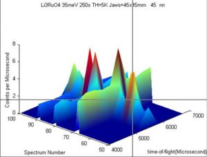
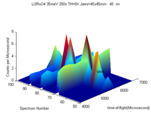
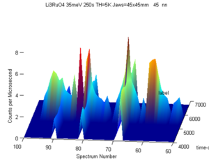
Finding and labelling points on a plot is done using the dxyz command. This can also place text on the plot at the desired point. A set of crosshairs will appear on the currently selected figure. By clicking on a point the x, y and z coordinates are found and returned through the function, any text is placed at the point.

>> dxyz
>> dxyz('text')
>> [x, y] = dxyz
>> [x, y, z] = dxyz
>> [x, y, z] = dxyz('text')
>> [x, y, z] = dxyz('property', value)
>> [x, y, z] = dxyz('text', 'propterty', value)

where 'property' and value relate to property-value pairs which are given below.

• By default, points will be returned until the return key is pressed on the keyboard
• If no output arguments are requested then the co-ordinates of the points are added as text at the point selected
• If text is given it is added to the plot (before the co-ordinates if they are to be added)
• If the plot is one dimensional then the returned z value will always be 0
• Function can be called without the z output
• If on a surface, the point chosen will be the (x,y,z) coordinate of the first face of the surface which intersects the selection ray (which is a "ray that goes into the screen). If no face intersects then NaN is returned.
• If on an area plot then the z value will be the intensity value of the pixel that was selected
• If on a [[Plot Commands#Two Dimensional Plots|multiplot] or one dimensional plot then the returned values will be the x,y,z points that corresponds to the closest data point on the closest intersecting face to the selection ray.

Optional Properties

Property	Possible Value	Behaviour	Default
'text'	Any string value	Text is added to the selected point	BLANK
'no_points'	Any numeric value	Defines the number of points that are to be selected on the plot. Once 'no_points' number of points have been sleected, the function will end. If left blank, this has the same as the default behaviour	Infinate
'display_coords'	True or False	If true, then the co-ordinates of the points selected will be placed on teh graph at the slected points. If text is given as well, the co-ordinates will be appended to the end of the text	False
'closest_point'	True or False	The co-ordinates of the closest actual point of the data is returned as the point	False

EXAMPLE:

>> [x,y,z] = dxyz('label')

The user will see

user clicks on point
user presses return

user rotates the view

EXAMPLE:

>> [x,y,z] = dxyz('text','mytext','display_coords',true,'no_points',5)

• x,y,z co-ordinates of 5 points will be recorded before the function stops
• 'mytext' (x, y, z) will be placed at each point, where x, y and z are the co-ordinates of the point
• The user may press return before all 5 points have been selected to end the function

Figure Control Functions

The figure windows can be controlled using name tags or the keep figure function. By default plots of the same type (one dimensional, surface, area, multiplot and sliceomatic appear in the same window and replace each other. The easiest way to get a handle on how this works is to play around with some simple plots.

However, if you want to keep the current plot and prevent any new plot replacing it, then use the command

>> kf

or

>> keep_figure

The title bar of the plot will now contain "(HOLD)" and any new plots will go to a new window. However, if a plot is on hold and you would like to use the figure to plot into again, then it can be released (the reverse of kf)

>> rf

or

>> release_figure

Using name tags is a little more complicated. Each figure has a name and tag (some default names and tags are used for various types of plot). Now windows are represented by their names and tags. For instance, a program that builds on top of libisis may have two plots that need to be permanently open and updated. By giving them two different names and/or tags, it is easy to keep track of which one will be updated. A script might be written such that

for i = 1:20
    monitor = get_monitor_function(i)
    data = get_data_function(i)
    dl (monitor, 'name','monitor1')
    dm (data, 'name', 'data')
    pause
end

Here, a user will see two plots, one titled 'monitor1', and the other titled 'data'. When the user clicks, a new monitor will replace the 'monitor1' figure window and new data will replace the 'data' figure window. The functions get_monitor_function and get_data_function are written by the user to get the data in the form of IXTdataset_1d objects.

Advanced Controls

The advanced controls are really intended for programming use. They perform the same functions as the basic Matlab controls set and get. However, the commands may be used with name tags and all three commands can be given either the figure, axes or plot handle related to the object in question. For instance

>> set_axes(ident, 'property', value)
>> set_plot(ident, 'property', value)
>> set_figure(ident, 'property', value)

OR names and tags can be used

>> set_plot('name', 'tag', 'property', value)

• Ident may be either figure, axes or plot handle
• set_axes with a figure handle will set the property 'property' to the value 'value' for all axes objects contained in the figure
• set_ axes with an axes handle will set the property 'property' to the value 'value' in the axes object
• set_axes with a plot handle will set the 'property' to the value 'value' for the parent axes of the plot
• set_figure with a figure object will set the 'property' to the value 'value' for the figure
• set_figure with axes or plot handle will set the 'property' to the value 'value' for the figure that contains that axes or plot
• set_plot with a figure or axes handle will set the 'property' to the value 'value' for all plots contained within the figure or axes given.
• set_plot with a plot handle will set 'property' to the value 'value' for the plot handle given
• Giving a name and tag is equivilent to giving a figure handle