Difference between revisions of "Plot Commands"
m |
m (→Plot Types) |
||
| Line 1: | Line 1: | ||
| − | |||
==One Dimensional Plots== | ==One Dimensional Plots== | ||
| Line 38: | Line 37: | ||
<pre>>> dh(w, 'property', value, 'property2', value2,...)</pre> | <pre>>> dh(w, 'property', value, 'property2', value2,...)</pre> | ||
| − | where w is a dataset | + | where w is a dataset, 'property' and value define [[General Behaviour#Property-Value Pairs|property-value pairs]]. See [[User Reference]] for list of properties that can be set |
===Overplots=== | ===Overplots=== | ||
Revision as of 08:43, 20 March 2008
One Dimensional Plots
Plot Types
Images of the one dimensional plot types can be seen here.
| Command | Plot Type |
|---|---|
| dl | Line Plot |
| dm | Marker Plot |
| de | Errorbar Plot |
| dh | Histogram Plot |
| dp | Marker with Errorbars Plot |
| dp | Marker and Line with Errorbars Plot |
Syntax:
>> dh(w, 'property', value, 'property2', value2,...)
where w is a dataset, 'property' and value define property-value pairs. See User Reference for list of properties that can be set
Overplots
If an overplot command is used, then the next plot will appear on top of the plot in the relevant plot window.
| Command | Plot Type |
|---|---|
| pl | Overplot Line |
| pm | Overplot Marker |
| pe | Overplot Errorbar |
| ph | Overplot Histogram |
| pp | Overplot Marker with Errorbars |
| pp | Overplot Marker and Line with Errorbars |
Plotting Arrays of IXTdataset_1d
If a one dimensional plot command is given an array of IXTdataset_1d objects then each IXTdataset_1d will be plotted as an overplot. Their order in the array is the same as the plotting order so that
>> dl(w, optional)
is the same as
for i = 1:length(ww)
    pl(w(i), optional)
end
EXAMPLE:
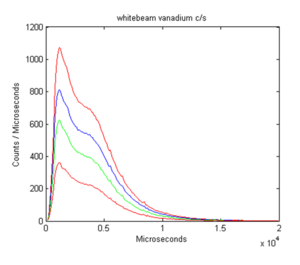
If w is a 4 element array of IXTdataset_1d objects then
>> acolor('red', 'blue', 'green')
>> dl(w)
Gives the following result
Plotting Arrays of IXTdataset_2d
When a one dimensional plot is made of an IXTdataset_2d object then the IXTdataset_2d object is expanded into an array of IXTdataset_1d objects and then plotted.
Two Dimensional Plots
Plot Types
Images of the two dimensional plot types can be seen here.
| Command | Plot Type |
|---|---|
| da | Area Plot |
| ds | Surface Plot |
| mp | Multiplot Plot |
Syntax:
>> ds(ww, 'property', value, 'property2', value2,...)
where w is a dataset and 'property' and value define property-value pairs. See the functions for a list of properties that can be set.
Plotting Arrays of IXTdataset_1d
An array of IXTdataset_1d objects is converted into an array of IXTdataset_2d objects and then plotted, if possible the IXTdataset_2d objects are contracted into a single IXTdataset_2d.
Plotting Arrays of IXTdataset_2d
Area Plot and Multiplot
These plot each dataset on top of the last. So if data from two datasets overlap in an area plot, then the plotted data will be taken from the latest in the array.
Surface Plot
A surface plot may be plotted in one of two different ways
- Combined (Default) - the data is combined and plotted as a single plot
- Separate - different plots are made on the same axis, one for each dataset
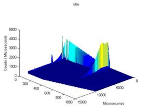
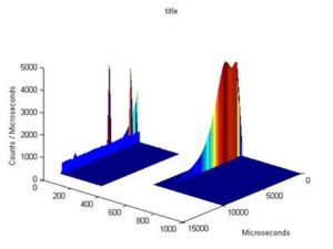
| &nsp | Combined | Separate |
|---|---|---|
| Description | A set of points evenly distributed between the minimum and maximum values of all data are chosen. Signal data are then interpolated accross these points using linear interpolation. | Data is plotted in the order it appears in the array. No interpolation is done. |
| Useful For | Data that originates from the same run but has been split into many IXTdataset_2d objects or an array of IXTdataset_1d objects | Separate data that is to be displayed side by side |
| Computational Time and Memory | Long time with high memory cost to perform the interpolation. Only possible on small arrays | Minimal resources used |
| Syntax | >> ds(ww) | >> ds(ww, 'separation', 'on') |
| Images | 
|

|
Three Dimensional Plots
Sliceomatic
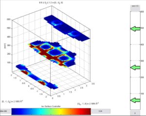
Sliceomatic is a special addition to the graphics package and is not fully implimented. Optional settings are severely limited and many commands simiply don't work with Sliceomatic. It is a stand alone application. However, keep_figure and name tags (see below) still work and are the most useful tools.
Syntax
>> sm(d3a, optional)
here, d3a is an IXTdataset_3d object.
Optional Inputs
All of the plotting commmadns accept similar optional input arguments. Below are a few examples, see here for a full list of optional inputs.
>> dl(w1, xlo, xhi, ylo, yhi)
>> dl(w1, xlo, xhi)
>> ds(ww, xlo, xhi, ylo, yhi, zlo, zhi)
>> dl(w, 'color','green','title','myplot')
>> da(w1, 'zlim', [0,0.1])
Using Name Tags
Names and Tags are used to identify plots and define properties for them. See here for more detailed information about properties and name tags.
Each plot with the same name and tag will have the same behaviour and default properties. They will plot into the same window (as long as it isn't on hold) and replace its contents. When setting properties pre-emptively name tags may be given so that only properties of certain plots are changed.
Syntax:
>>dl(w1, 'name', 'myname', 'tag', 'mytag')
By default each plot type has a different name and all tags are blank
| Plot Type | Default Name |
|---|---|
| Oned (histogram, line, errorbar and marker) | 'default one dimensional plot' |
| Area | 'default area plot' |
| Surface | 'default surface plot' |
| Multiplot | 'default multiplot' |
| Sliceomatic | 'Sliceomatic' |
Therefore, by default, each of these plot types will have their own figure window when plotting, but plots of the same type will replace each other unless they are held.

